Unloading Stiffness Fit

This example shows how the unloading part of a force-depth curve is fitted to obtain the contact stiffness used by the Oliver-Pharr method.

import matplotlib.pyplot as plt
import numpy as np

from micromechanics.indentation import Indentation
from micromechanics.indentation.definitions import Method

Build a compact synthetic load-unload experiment. The loading segment rises linearly, while the unloading segment follows a power law with a known residual depth. The synthetic data makes it easy to see which part of the curve is used for the stiffness fit.

loading_depth = np.linspace(0.0, 1.0, 24)
loading_force = np.linspace(0.0, 5.0, 24)
unloading_depth = np.linspace(1.0, 0.25, 36)
unloading_force = 5.0*((unloading_depth-0.1)/(1.0-0.1))**1.5

depth = np.r_[loading_depth, unloading_depth]
force = np.r_[loading_force, unloading_force]

iLHU stores the load-hold-unload indices as [load start, load end, unload start, unload end]. Real instrument files populate this during loading or with identifyLoadHoldUnload.

indentation = Indentation("")
indentation.method = Method.ISO
indentation.setRawData(depth, force, np.arange(len(depth), dtype=float))
indentation.iLHU = [[0, len(loading_depth)-1, len(loading_depth), len(depth)-1]]
indentation.output["verbose"] = 3

*WARNING*: Poisson Ratio different than in file. 0.3 0.18
Open Agilent file: /home/runner/work/micromechanics/micromechanics/micromechanics/indentation/data/Example.xls

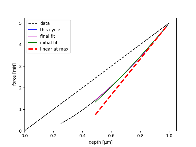
The fitting routine returns the stiffness, a mask marking the evaluated point, the unloading-fit mask, the optimized power-law parameters, and a success flag.

stiffness, valid, mask, opt, powerlaw_fit = indentation.stiffnessFromUnloading(force, depth, plot=True)
print(f"Fitted unloading stiffness: {stiffness[0]:.2f} mN/um")
print(f"Power-law fit succeeded: {powerlaw_fit[0]}")

Number of unloading segments:1  Method:1
Initial fitting values B,hf,m 6.755229140733971 0.21344081076517907 1.2589254117941673
  Bounds (array([0. , 0. , 0.8]), array([        inf,  0.67857143, 10.        ]))
  Optimal values B,hf,m 5.856069741415784 0.1000000000415452 1.4999999999144056
Fitted unloading stiffness: 8.33 mN/um
Power-law fit succeeded: True

The red dashed line in the figure is the tangent stiffness. This is the slope that later enters the Oliver-Pharr contact-depth and modulus calculation.

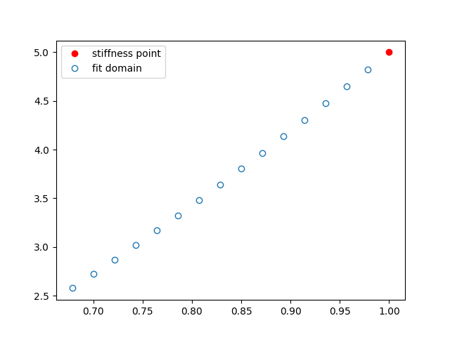
plt.plot(depth[valid], force[valid], "ro", label="stiffness point")
plt.plot(depth[mask], force[mask], "C0o", fillstyle="none", label="fit domain")
plt.legend()

<matplotlib.legend.Legend object at 0x7fda2e4dc550>