Tip Area Models

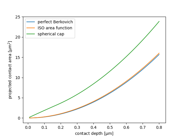
This example compares projected contact area for a perfect Berkovich tip, an ISO-style calibrated area function, and a spherical tip.

import matplotlib.pyplot as plt
import numpy as np

from micromechanics.indentation import Tip

The projected contact area is evaluated as a function of contact depth. All depths passed to areaFunction are in micrometers, while the calibrated prefactors are stored in the unit convention used by the indentation package.

contact_depth = np.linspace(0.01, 0.8, 120)

A perfect Berkovich tip is the usual analytical reference. The ISO-style tip uses a polynomial area function, and the spherical model is useful for blunt tips or rounded apex behavior at shallow depth.

perfect = Tip("perfect")
iso = Tip(shape=[24.5, 420.0, -30.0])
sphere = Tip(shape=[3.0, 70.3, "sphere"])

Larger area at a given depth means the same load would produce a lower hardness. Comparing area functions is therefore a direct way to inspect how a tip calibration changes the mechanical result.

area_perfect = perfect.areaFunction(contact_depth.copy())
area_iso = iso.areaFunction(contact_depth.copy())
area_sphere = sphere.areaFunction(contact_depth.copy())

fig, ax = plt.subplots()
ax.plot(contact_depth, area_perfect, label="perfect Berkovich")
ax.plot(contact_depth, area_iso, label="ISO area function")
ax.plot(contact_depth, area_sphere, label="spherical cap")
ax.set_xlabel(r"contact depth [$\mathrm{\mu m}$]")
ax.set_ylabel(r"projected contact area [$\mathrm{\mu m^2}$]")
ax.legend()

<matplotlib.legend.Legend object at 0x7fda32b07c50>

The inverse area function maps a measured contact area back to contact depth.

known_area = perfect.areaFunction(np.array([0.35]))
recovered_depth = perfect.areaFunctionInverse(known_area)
print(f"Use initial depth 0.35um and recovered depth for the perfect tip: {recovered_depth[0]:.3f} um")

Use initial depth 0.35um and recovered depth for the perfect tip: 0.350 um