Tif Processing Steps

This example applies common processing steps to a Zeiss SEM TIF image and compares the intermediate results.

from pathlib import Path

import matplotlib.pyplot as plt

import micromechanics
from micromechanics.tif import Tif

repository_root = Path(micromechanics.__file__).resolve().parents[1]
file_name = repository_root / "examples" / "Zeiss" / "Zeiss.tif"

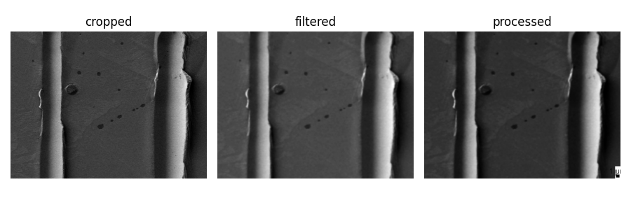
Load the Zeiss SEM image and crop to a region of interest. Keeping a copy after each stage makes it easy to compare the effect of each processing step.

image = Tif(str(file_name))
image.crop(xMin=50, xMax=450, yMin=50, yMax=350)
cropped = image.image.copy()

After cropping: new size of image:  400 300

Apply a median filter to suppress isolated pixel noise, then a Gaussian filter for mild smoothing. The two filters target different kinds of image noise.

image.medianFilter(level=2)
image.gaussFilter(level=1)
filtered = image.image.copy()

Adjust contrast and add a scale bar. The processed copy is the version that would typically be used in a figure or report.

image.contrast(magnitude=1.4, offset=0.45, save=True)
image.addScaleBar(site="BR", length=1)
processed = image.image.copy()

Compare the intermediate results side by side. This helps tune the crop, filtering, and contrast parameters before saving a final image.

fig, axes = plt.subplots(1, 3, figsize=(9, 3))
for ax, title, data in zip(axes,
                          ["cropped", "filtered", "processed"],
                          [cropped, filtered, processed]):
  ax.imshow(data, cmap="gray")
  ax.set_title(title)
  ax.axis("off")

plt.tight_layout()