Hertz Contact Fit

This example creates an ideal elastic loading segment for a spherical indenter, adds a small displacement offset, and fits the first part of the curve with the Hertz contact equation.

import matplotlib.pyplot as plt
import numpy as np

from micromechanics.indentation import Indentation
from micromechanics.indentation.hertz import hertzEquation

Start from an empty Indentation object. In a real workflow the depth and force arrays would usually come from an instrument file. Here they are generated explicitly so the fitted contact point and modulus are known.

indentation = Indentation("")
indentation.output["verbose"] = 2

*WARNING*: Poisson Ratio different than in file. 0.3 0.18
Open Agilent file: /home/runner/work/micromechanics/micromechanics/micromechanics/indentation/data/Example.xls

The Hertz equation describes elastic contact between a spherical indenter and a flat sample. true_h0 shifts the apparent zero of depth, which mimics the practical problem of finding the first physical contact point.

true_h0 = 0.018
true_reduced_modulus = 9500.0
depth = np.linspace(0.0, 0.18, 80)
force = hertzEquation(depth.copy(), true_h0, true_reduced_modulus)

Assign the synthetic loading curve to the indentation object and fit only the low-load elastic part of the curve. The force range should be chosen before plastic deformation or pop-in events dominate the response.

indentation.setRawData(depth.copy(), force.copy(), np.arange(len(depth), dtype=float))

fit_h0, fit_reduced_modulus = indentation.hertzFit(forceRange=(0.02, 6.0), correctH=False, plot=False)

Depth range (0.018227848101265823, 0.02278481012658228)
Optimal parameters (h0,prefactor) [1.8e-02 9.5e+03]

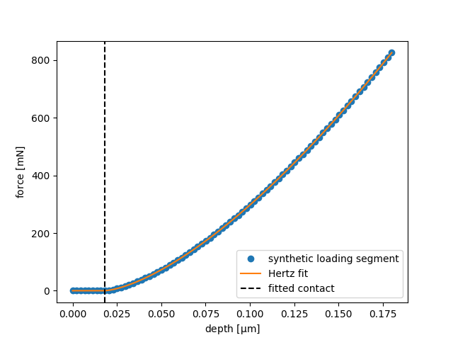
Plot the measured curve and the fitted Hertz curve. The dashed line marks the recovered contact point; for this synthetic data it should coincide with the known offset used above.

fit_depth = np.linspace(depth.min(), depth.max(), 200)
fit_force = hertzEquation(fit_depth.copy(), fit_h0, fit_reduced_modulus)

fig, ax = plt.subplots()
ax.plot(depth, force, "o", label="synthetic loading segment")
ax.plot(fit_depth, fit_force, "-", label="Hertz fit")
ax.axvline(fit_h0, color="k", linestyle="dashed", label="fitted contact")
ax.set_xlabel(r"depth [$\mathrm{\mu m}$]")
ax.set_ylabel(r"force [$\mathrm{mN}$]")
ax.legend()

<matplotlib.legend.Legend object at 0x7fda32b04050>