SEM Gray-Value Gradient Correction

This example builds a small SEM-like grayscale image with an illumination gradient and compares two correction methods used for cross-section images.

from pathlib import Path
from tempfile import TemporaryDirectory

import matplotlib.pyplot as plt
import numpy as np
from PIL import Image

from micromechanics.tif import Tif

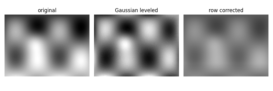
Build a small synthetic SEM-like image. The sinusoidal term gives texture, the Gaussian spot represents a brighter feature, and the linear term creates the unwanted vertical illumination gradient.

y, x = np.mgrid[0:160, 0:220]
matrix = 90 + 40*np.sin(x/18.0)*np.sin(y/24.0)
particles = 55*np.exp(-((x-80)**2+(y-70)**2)/(2*18**2))
illumination = 0.42*y
image_array = np.clip(matrix + particles + illumination, 0, 255).astype(np.uint8)

Tif normally reads instrument files from disk, so the synthetic image is written to a temporary TIF first. fileType="Conventional" skips vendor metadata parsing and uses the given pixel size directly.

with TemporaryDirectory() as tmp:
  file_name = Path(tmp) / "synthetic_sem.tif"
  Image.fromarray(image_array).save(file_name)

  original = Tif(str(file_name), fileType="Conventional", pixelSize=0.02)

  #############################################################################
  # ``gaussLevel`` estimates a smooth background using a Gaussian filter and
  # subtracts it. This is useful when the illumination variation is broad
  # compared with the microstructural features.

  leveled = Tif(str(file_name), fileType="Conventional", pixelSize=0.02)
  leveled.gaussLevel(level=18, plot=False, save=True)

  #############################################################################
  # ``removeGrayGradient`` fits a row-wise intensity trend and subtracts only
  # positive excess brightness. This targets cross-section images where one
  # direction carries most of the gray-value drift.

  row_corrected = Tif(str(file_name), fileType="Conventional", pixelSize=0.02)
  row_corrected.removeGrayGradient(save=True, plot=False)

/home/runner/work/micromechanics/micromechanics/micromechanics/tif/processing.py:297: RankWarning: Polyfit may be poorly conditioned
  myFit = np.polyfit(x[maxYsum:], ysum[maxYsum:],2)

Compare the unprocessed image with both corrections. The best choice depends on whether the gradient is broad and two-dimensional or primarily row-wise.

fig, axes = plt.subplots(1, 3, figsize=(9, 3))
for ax, title, data in zip(axes,
                          ["original", "Gaussian leveled", "row corrected"],
                          [original.image, leveled.image, row_corrected.image]):
  ax.imshow(data, cmap="gray")
  ax.set_title(title)
  ax.axis("off")
plt.tight_layout()