Tutorial EBSD

The examples demonstrate how to read EBSD files, plot inverse pole figures, and interact with the data in the file.

Example: Read EBSD data and plot the ND IPF

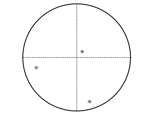
Let’s looking at inverse pole figure (IPF) in normal direction (ND) and pole-figure (PF) in the [1,0,0] direction.

• Read EBSD data from a file (e.g., .ang, .osc, .crc, or .txt).

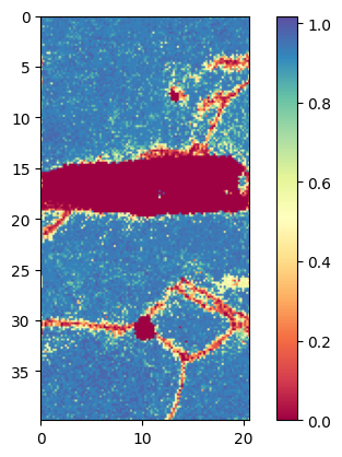
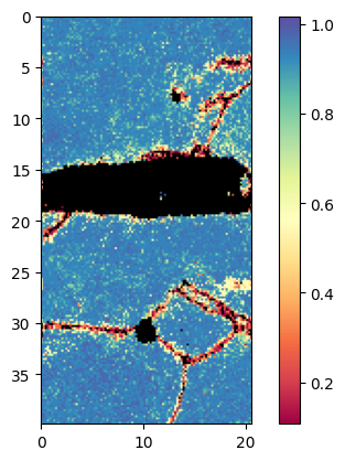
• Plot confidence index (CI). Mask out all points with a CI less than 0.1. Initially all points are present in the mask, i.e. they are shown. By masking out points, these are removed from the mask.

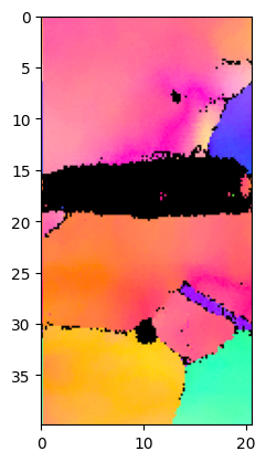
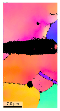
• Plot inverse pole figure in normal direction

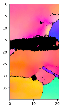
• Play with different options (e.g. 1024 pixel to see speed of plotting)

• setVMask: for fast plotting

• Pole figure (PF) in the [1,0,0] direction. The OIM software has the top left corner as coordinate origin

from ebsdlab.ebsd import EBSD
e = EBSD("../tests/DataFiles/EBSD.ang")
print('\nPlot confidence index:')
e.plot(e.CI)
print('\nPlot confidence index with mask:')
e.maskCI(0.1)
e.plot(e.CI)
print('\nPlot default IPF:')
e.plotIPF()
print('\nPlot IPF with 1024 pixel resolution:')
e.plotIPF(1024)
e.addScaleBar()
e.setVMask(4)  # use only every 4th point, increases plotting speed
print('\nPlot IPF with scale-bar and with 1024 pixel resolution:TODO')
e.plotIPF(1024)
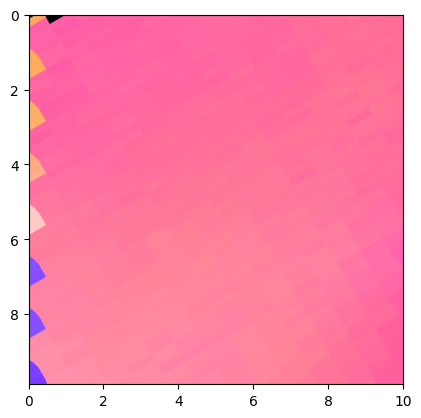
print('\nPlot IPF of the cropped area with 1024 pixel resolution:')
e.cropVMask(0,0,10,10)  # show only a section of the image, increases plotting speed
e.plotIPF(1024)
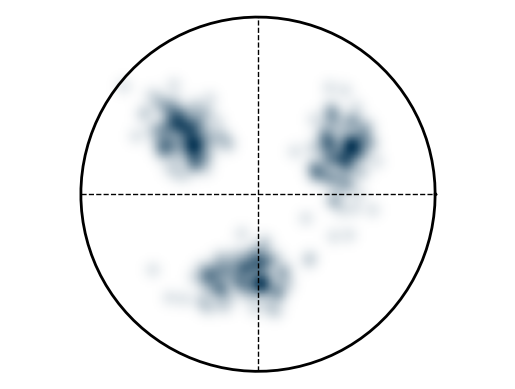
print('\nPlot PF as a density:')
e.plotPF([1,0,0])
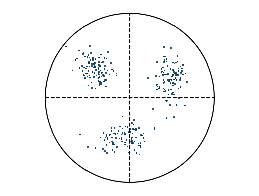
print('\nPlot PF as points:')
e.plotPF([1,0,0], points=True)

Load .ang file:  ../tests/DataFiles/EBSD.ang
   Read file with step size: 0.2 0.2
   Optimal image pixel size: 103
   Number of points: 23909
   Duration init:  0 sec

Plot confidence index:
   Plot with x and y axis in [um]
Duration plot:  0 sec

Plot confidence index with mask:

   Plot with x and y axis in [um]
Duration plot:  0 sec

Plot default IPF:

Duration plotIPF:  0 sec

Plot IPF with 1024 pixel resolution:

Duration plotIPF:  3 sec

Plot IPF with scale-bar and with 1024 pixel resolution:TODO

Duration plotIPF:  2 sec

Plot IPF of the cropped area with 1024 pixel resolution:

Duration plotIPF:  1 sec

Plot PF as a density:
Duration plotPF:  0 sec

Plot PF as points:
Duration plotPF:  0 sec

Example: Interaction with OIM Software to update grain information

Note

This example is worthwhile. However, the TestB.txt file is not included in the repository. Recreate it

This example demonstrates how to process an OIM data file using this Python library and subsequently export the modified data for re-import into the OIM software.

1. How to export txt-file from OIM that can be imported into this python library:

   • Partition->export-> grain file -> use “grain file type 1” (saves a txt file)

   • Partition->export-> partition data -> save as .ang

2. Process with python: remove some masked points:

   e = EBSD("../tests/DataFiles/Test.ang")
   e.loadTXT("../tests/DataFiles/TestB.txt")
   e.maskCI(0.1)
   e.removePointsOfMask()
   e.writeANG("ebsd.ang")
   

3. Which can then be read in OIM again.

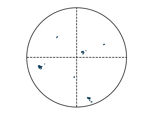
Example: Create artificial EBSD pattern

This example generates an artificial EBSD pattern, where parameters are separated by “|”: - The first three values specify the grain orientation as Euler angles. - The fourth value defines the standard deviation around the mean orientation. - The fifth value specifies the number of points to generate.

from ebsdlab.ebsd import EBSD
e = EBSD('void318.|125.|219.6|0.2|10')
e.plotPF(size=5)
e.plotPF(points=True)

Void mode 318.|125.|219.6|0.2|10
   Euler angles: 5.55 2.18 3.83 | distribution: 0.2 | numberPerAxis: 10.0
   Read file with step size: 1.0 1.0
   Optimal image pixel size: 9
   Number of points: 100
   Duration init:  0 sec
Duration plotPF:  0 sec

Duration plotPF:  0 sec

Example: Average orientation in file

Compute the mean grain orientation for all points in the map.

• The operation Orientation.average() is computationally intensive.

• Averaging orientations across multiple grains is not physically meaningful, but is shown here for demonstration purposes.

import numpy as np
from ebsdlab.orientation import Orientation
from ebsdlab.ebsd import EBSD
Orients = []
e = EBSD("../tests/DataFiles/EBSD.ang")
for i in range(len(e.x)):
    Orients.append(Orientation(quaternion=e.quaternions[i], symmetry="cubic"))
avg = Orientation.average(Orients)
print("Average orientation", np.round(avg.asEulers(degrees=True, standardRange=True), 0))

Load .ang file:  ../tests/DataFiles/EBSD.ang

   Read file with step size: 0.2 0.2
   Optimal image pixel size: 103
   Number of points: 23909
   Duration init:  0 sec

Average orientation [ 79.  10. 282.]